Here I’ll give the theory part of Neural Networks, sepecifically three kinds of NN: Normal Neural Networks, Convolutional Neural Networks, Recurrent Neural Networks.
Neural Networks
In single neuron:
$$\begin{align*} z &= Wx + b \\ a &= \sigma (z) \end{align*}$$Activation Function
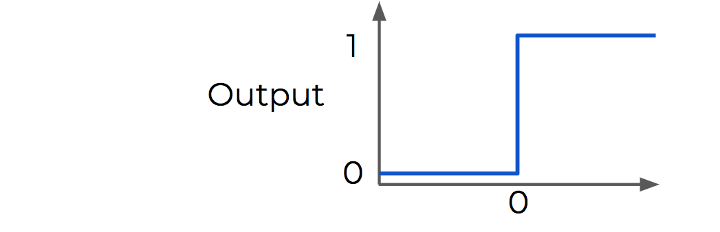
- Perceptron: binary classifier, small changes are not reflected.$$\begin{align*} f(x) = \begin{cases} 1 & \text{if } Wx+b>0\\ 0 & \text{otherwise} \end{cases} \end{align*}$$
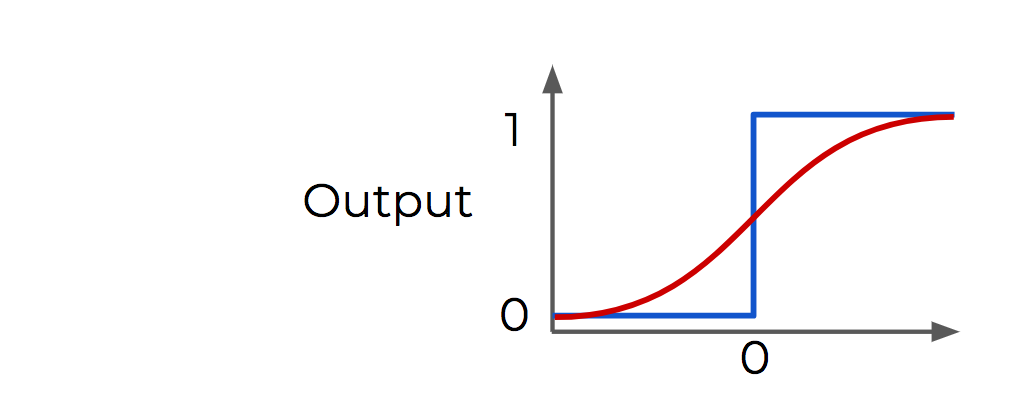
Sigmoid: special case of the logistic function with S shape curve, more dynamic
$$\begin{align*} S(x) = \frac{1}{1 + e^{-x}} = \frac{e^x}{e^x +1} \end{align*}$$
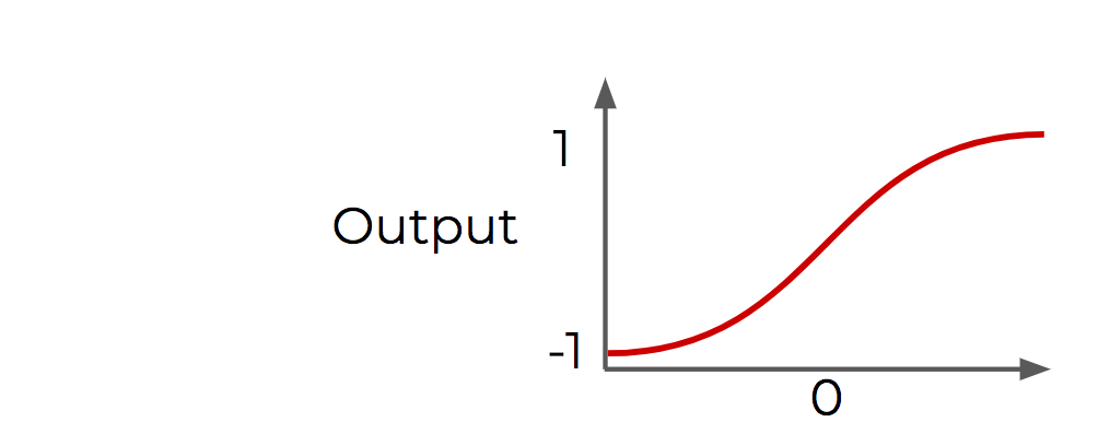
$$\begin{align*} cosh x &= \frac{e^x + e^{-x}}{2}\\ sinh x &= \frac{e^x - e^{-x}}{2}\\ tanh x &= \frac{cosh x}{sinh x } \end{align*}$$
ReLU (Rectified Linear Unit): max(0,z)
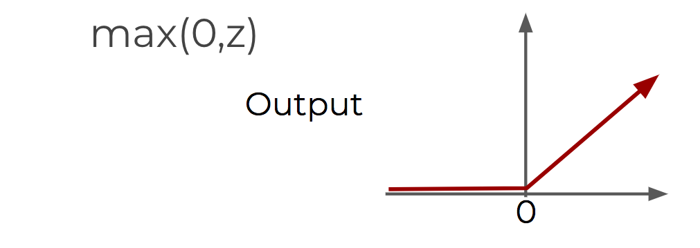
ReLU and tanh tend to have the best performance.Softmax Regression:
$$\begin{align*} z_i &= \sum_jW_{i,j}x_j + b_i \\ softmax(z)_i &= \frac{\text{exp}(z_i)}{\sum_j \text{exp}(z_j)} \end{align*}$$
Cost/Loss Function
Cost function is the measurement of the error.
$$\begin{align*}
z &= Wx + b \\
a &= \sigma (z)\\
C &= \frac{1}{n}\sum(y_{true} - a)^2 &\text{Quadratic Cost}\\
C &= -\frac{1}{n}\sum(y_{true}\cdot ln(a) + (1-y_{true})\cdot ln(1-a) ) &\text{Cross Entropy}
\end{align*}$$
Quadratic Cost:
The larger errors are more prominent due to the squaring. It causes a slowdown in learning speed.
Cross Entropy:
It allows for faster learning. The larger the difference, the faster the neuron can learn.
Gradient Descent & Backpropagation
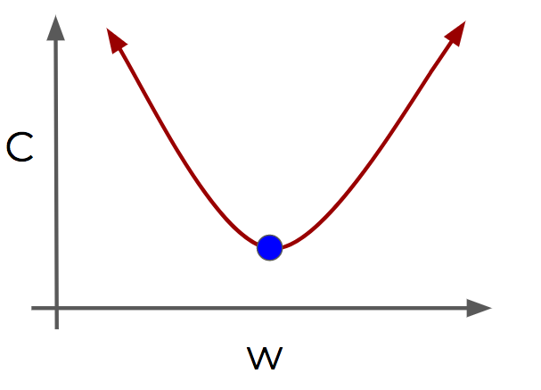
Gradient Descent is an optimization algorithm for finding the minimum of a function. Here it minimizes the error to find the optiml value. 1-D example below shows the best parameter value (weights of the neuron inputs) we should choose to minimize the cost.
For complicated cases more than 1 dimension, we use biilt-in algebra of Deep learning library to get the optimal parameters.
1. Learning Rate: defines the step size during gradient descent, too small - slow pace, too small - overshooting
2. Batch Size: batches allow us to use stochastic gradient descent, in case the datasets are large, if all the them are fed at once the computation would be very expensive. Too small - less representative of data, too large - longer training time
3. Second-Order Behavior of Gradient Descent: adjust the learning rate based on the rate of descent(second-order behavior: derivative),large learning rate at the beginning, adjust to slower learning rate as it get closer. Methods: AdaGrad, RMSProp, Adam
Vanishing Gradients: when increasing the number of layers in a network, the layers towards the input will be affected less by the error calculation occuring at the output as going backwards throught the network. Initialization and Normalization will help to mitigate the issue.
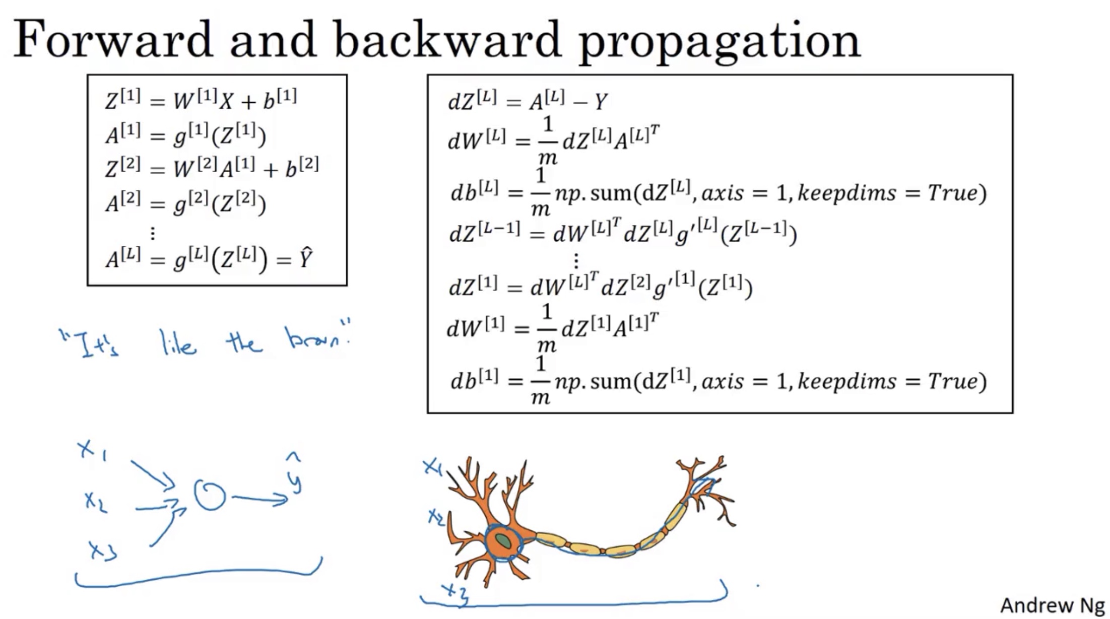
Backpropagation is to calculate the error contribution of each neuron after a batch of data is processed. It works by calculating the error at the output and then distributes back through the network layers. It belongs to supervised learning as it requires a known output for each input value. The mathematical detail is showed below from Andrew Ng’s Neural Networks and Deep Learning in Coursera.
Initialization of Weights
Zeros
No randomness (too subjective) so not a good choice
Random Distribution
Random distribution near zero is not optimal and results in activaion function distorition (distorted to large values)
Xavier (Glorot) Initialization
The weights drawn from uniform or normal distribution, with zero mean and specific variance $\text{Var}(W) =\frac{1}{n_{in}} $:
$$\begin{align*}
&Y = W_1X_1 +W_2X_2 + ... + W_nX_n\\
&\text{Var}(W_iX_i) = E[X_i]^2\text{Var}(W_i) + E[W_i]^2\text{Var}(X_i) + \text{Var}(W_i)\text{Var}(X_i)\\
&\text{Var}(W_iX_i) = \text{Var}(W_i)\text{Var}(X_i) \qquad (\because E[X_i] = 0)\\
&\text{Var}(Y) = \text{Var}(W_1X_1 + W_2X_2 +... + W_nX_n) = n \text{Var}(W_i)\text{Var}(X_i) \\
&\because \text{Variance of the output is equal to the variance of the input}\\
&\therefore n\text{Var}(W_i) = 1\\
&\therefore \text{Var}(W_i) = \frac{1}{n} = \frac{1}{n_{in}} = \frac{2}{n_{in} + n_{out} }
\end{align*}$$
Overfitting Issue
With potentially hundreds of parameters in a deep learning neural network, the possibility of overfitting is very high. We can mitigate this issue by the following ways:
- $L_1/L_2$ Regularization
Add a penalty for a larger weights in the model (not unique to neural networks) - Dropout
Remove neurons during training randomly so that the network does not over rely on any particular neuron (unique to neural networks) - Expanding Data
Artificially expand data via adding noise, tilting images
Convolutional Neural Networks
Tensor
Tensor: N-dimensional arrays:
Scalar: 3
Vector: [3,4,5]
Matrix: [[3,4],[5,6],[7,8]]
Tensor: [[[1,2], [3,4]], [[5,6], [7,8]]]
We use tensors to feed in sets of images into the model - (I,H,W,C)
I: Images
H: Height of Image in Pixels
W: Width of Image in Pixels
C: Color Channels: 1 - Grayscale, 3 - RGB
DNN vs CNN
Convolution
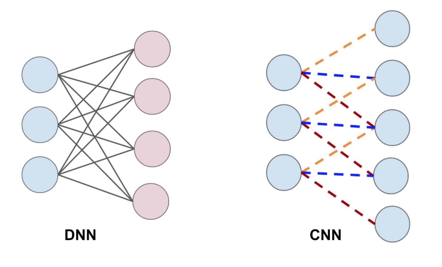
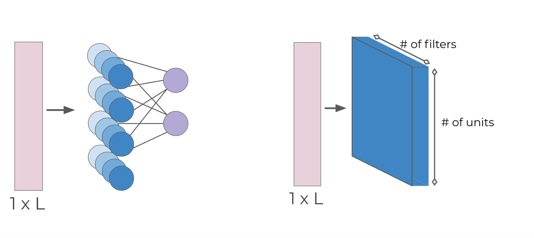
The left figure is densely connected layer, every neuron in the layer is directly connected to the every neuron in the next layer. While each unit in the convolutional layer is connected to a smaller number of nearby units in the next layer.
The reason for the idea of CNN is that most images are at least 256 by 256 pixels or greater (MNIST only 28 by 29 pixels, 784 total). So there are too many parameters unscalable to new images. Another merit of CNN is for image processing, pixels nearby to each other are much more correlated to each other for image detection. Each CNN layer looks at an increasingly larger part of the image. And having units only connected to nearby units helps invariance. CNN helps limit the search of weights to the size of the convolution. Convolutional layers are only connected to pixels in their respective fields. By adding a padding of zeros around the image we can fix the issue for edge neurons where there may not be an input for them.
Take the example of 1-D Convolution, we treat the weights as a filter for edge detection, then expand one filters to multiple filters. Stride 1 means 1 unit at a time. The top circle means the zero padding added to include more edge pixels. Each filter detects a different feature.
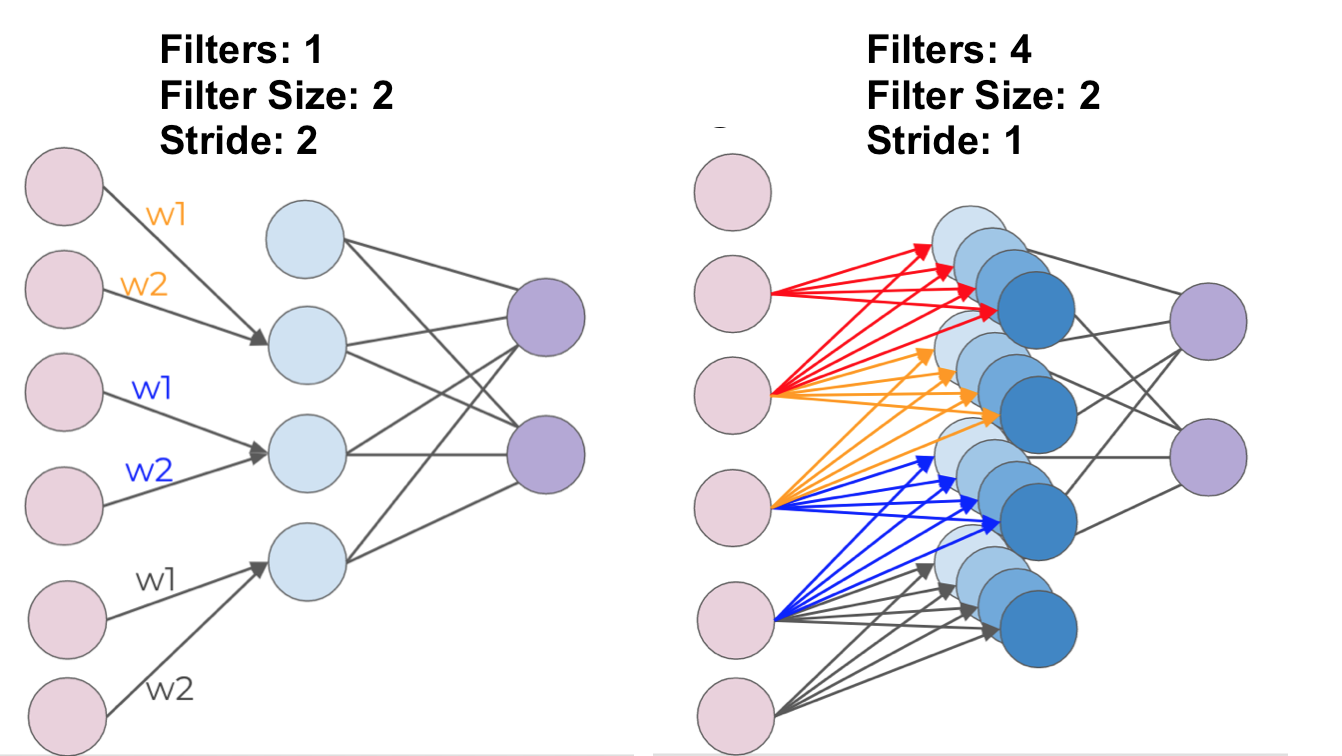
Now for simplicity, the sets of neurons are visualized as blocks.
For 2-D Images and Color Images:
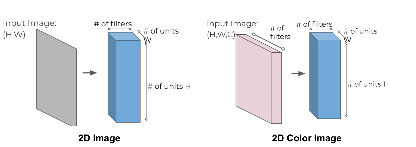
More Info: Image Kernals
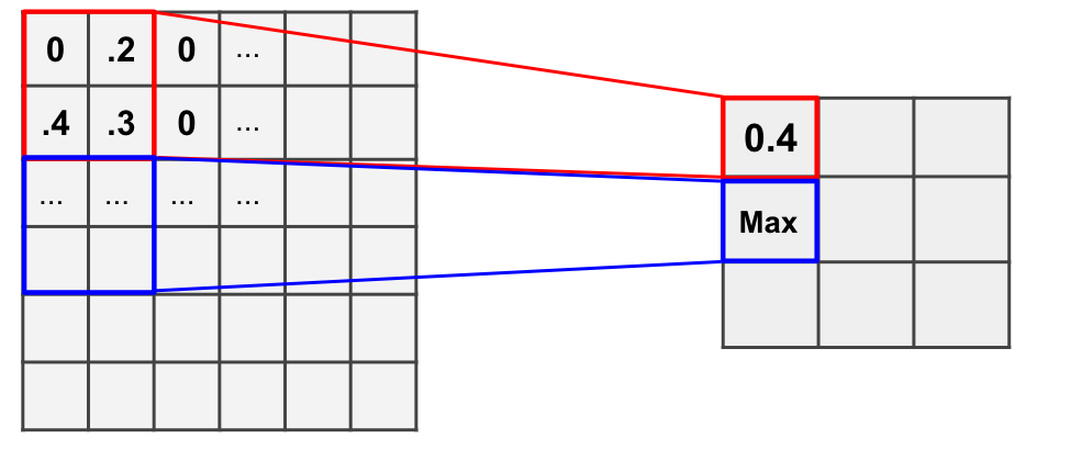
Subsampling
Except convolutional layers, there’s another kind of layers called pooling layers. Pooling layers will subsample the input image to reduce the memory use and computer load as well as reducing the number of parameters.
Take example of MNIST, only select max value to the next layer, and move over by stride. So the pooling layer will finally remove a lot of information.
Another technique is “Dropout”. Dropout is regarded as a form of regularization as during training, units are randomly dropped with their connection to help prevent overfitting.
Recurrent Neural Networks
Common Neural Networks can handle classification and regression problems, but for sequence information, we need Recurrent Neural Networks.
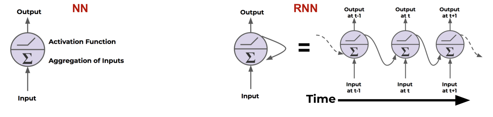
Normal Neural Networks just aggregation of inputs and pass the activation function to get the output. Recurrent Neural Networks send output back to itself.
Here I have to mention my previous research work – Echo State Networks, also belong to RNN: ESN
Cells that are a function of inputs from previous time steps are also know as memory cells.