defnext_batch(self, batch_size, steps, return_batch_ts = False): # grab a random starting point for each batch random_start = np.random.rand(batch_size,1) # convert the data to TS ts_start = random_start * (self.xmax - self.xmin - (steps * self.resolution)) # create batch time series on the x axis batch_ts = ts_start + np.arange(0.0,steps+1) * self.resolution # create the Y data for the time series x axis from previous step y_batch = np.sin(batch_ts) # formatting for RNN if return_batch_ts: return y_batch[:,:-1].reshape(-1,steps,1), y_batch[:,1:].reshape(-1,steps,1), batch_ts else: return y_batch[:,:-1].reshape(-1,steps,1), y_batch[:,1:].reshape(-1,steps,1) # original y_batch and y_batch shifted over 1 step in the future
1
2
3
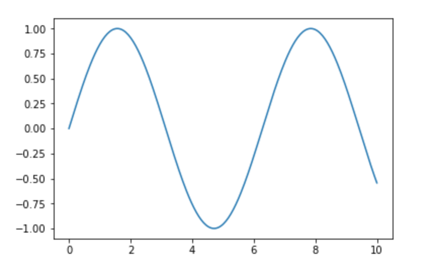
# Give the data and try the model!
ts_data = TimeSeriesData(250,0,10)
plt.plot(ts_data.x_data, ts_data.y_true)
1
2
3
4
5
6
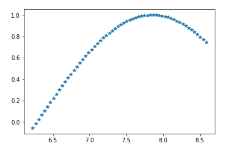
num_time_steps = 60
# Set 1 batch, 60 steps, return batch time series on x axis
y1, y2, ts = ts_data.next_batch(1, num_time_steps, True)
plt.plot(ts.flatten()[1:], y2.flatten(), '*')
# ts.flatten(): Return a copy of the array collapsed into one dimension.
# ts has total 251 points (including the prediction), so start from 1, to match y2
1
2
3
4
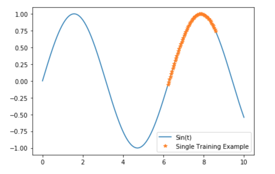
plt.plot(ts_data.x_data, ts_data.y_true, label ='Sin(t)')
plt.plot(ts.flatten()[1:], y2.flatten(), '*', label = 'Single Training Example')
plt.legend()
plt.tight_layout()   # Automatically adjust subplot parameters to give specified padding.
1
2
3
4
5
6
7
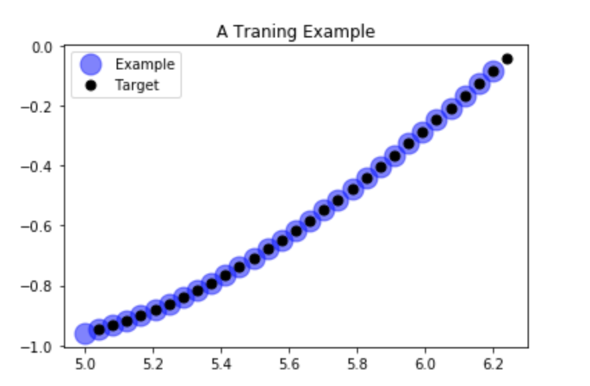
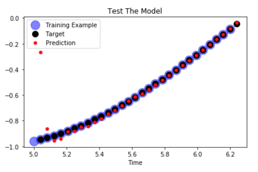
# Demonstrate what's going on of the training in the model, shift over 1 step
num_time_steps = 30
train_example = np.linspace(5, 5+ts_data.resolution*(num_time_steps + 1), num_time_steps + 1)
plt.title('A Traning Example')
plt.plot(train_example[:-1], ts_data.ret_true(train_example[:-1]), 'bo', markersize = 15, alpha = 0.5, label = 'Example')
plt.plot(train_example[1:], ts_data.ret_true(train_example[1:]), 'ko', markersize = 7, label = 'Target')
plt.legend()
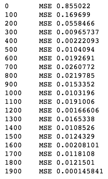
To further explore the performance of RNN model, we can change the number of iteration num_train_iterations, learning rate learning_rate, and model type tf.contrib.rnn.BasicRNNCell() and then play with it.
About just for time sequence that shifts 1 time step ahead, now we’ll generate a completely new sequence.
1
2
3
4
5
6
7
8
9
10
11
12
13
14
15
with tf.Session() as sess: saver.restore(sess, './rnn_time_series_model_codealong')
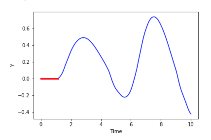
# seed zeros # 30 0s and the generated data zero_seq_seed = [0.0for i in range(num_time_steps)] for iteration in range(len(ts_data.x_data) - num_time_steps): X_batch = np.array(zero_seq_seed[-num_time_steps:]).reshape(1, num_time_steps,1) y_pred = sess.run(outputs, feed_dict = {X: X_batch}) zero_seq_seed.append(y_pred[0,-1,0]) plt.plot(ts_data.x_data, zero_seq_seed, 'b-') plt.plot(ts_data.x_data[:num_time_steps], zero_seq_seed[:num_time_steps], 'r', linewidth =3) plt.xlabel('Time') plt.ylabel('Y')
Instead of zeros at the beginning, now use training example, other parts remain the same
1
2
3
4
5
6
7
8
9
10
11
12
13
14
with tf.Session() as sess:
    saver.restore(sess, './rnn_time_series_model_codealong')

    # 30 training points and the generated data
    training_example = list(ts_data.y_true[:30])
    for iteration in range(len(ts_data.x_data) - num_time_steps):
        X_batch = np.array(training_example[-num_time_steps:]).reshape(1, num_time_steps,1)
        y_pred = sess.run(outputs, feed_dict = {X: X_batch})
        training_example.append(y_pred[0,-1,0])

plt.plot(ts_data.x_data, training_example, 'b-')
plt.plot(ts_data.x_data[:num_time_steps], training_example[:num_time_steps], 'r', linewidth =3)
plt.xlabel('Time')
plt.ylabel('Y')