I’m learning how to use Google’s TensorFlow framework to create artificial neural networks for deep learning with Python from Udemy. I’m using Jupiter notebook to practice and blog my learning progress here.
TensorFlow is an open source software library for numerical computation using data flow graphs. Nodes in the graph represent mathematical operations, while the graph edges represent the multidimensional data arrays (tensors) communicated between them. This architecture allows users to deploy computation to one or more CPUs or GPUs, in a desktop, server, or mobile device with a single API (Application programming interface).
Install TensorFlow Environment
Download Anaconda Distribution for Python 3.6 Version. Tutorial comes in that page.
For MacOS: Open Terminal, use cd to the target directory
Create the environment file: run conda env create -f tfdl_env.yml
Activate the file: run source activate tfdeeplearning
Now you are in the virtual environment of tfdeeplearning
If you want to get out of this, run source deactivate
Note: How is Anaconda related to Python?
Anaconda is a python and R distribution. It aims to provide everything you need (python wise) for data science “out of the box”.
It includes:
- The core python language
- 100+ python “packages” (libraries)
- Spyder (IDE/editor - like pycharm) and Jupyter
conda, Anaconda’s own package manager, used for updating Anaconda and packages
Also Anaconda is used majorly for the data science. which manipulates large datasets based on statistical methods. ie. Many statistical packages are already available in anaconda libraries(packages)
Vanilla python installed from python.org comew with standard library is okay, in which case using pip to install manually (which comes with most python dists and you should have it if you downloaded from python.org).
Learn more: Anaconda overview; Python 3 tutorial
TensorFlow Basic Syntax
1 | import tensorflow as tf |
Output: 1.3.0
Create a tensor ($\approx$ n-dimension array), the basic one (constant)1
2
3hello = tf.constant('Hello')
world = tf.constant('World')
type (hello)
Output: tensorflow.python.framework.ops.Tensor
Run this operation inside of a session:1
2
3with tf.Session() as sess:
result = sess.run(hello + world)
print(result)
Output: b'HelloWorld'
Note:
Use with is to make sure we don’t close the session until we run a block of code then close the session.
The b character prefix signifies that HelloWorld is a byte string, use result.decode('utf-8') to convert byte str to str.
1 | a = tf.constant(10) |
Output: 30
Numpy Operations:1
2
3
4
5
6
7
8
9
10
11
12const = tf.constant(10) # constant operation
fill_mat = tf.fill((4,4),10) # matrix operation 4x4
myzeros = tf.zeros((4,4)) # 4x4 zeors
myones = tf.ones((4,4)) # 4x4 ones
myrandn = tf.random_normal((4,4), mean = 0, stddev = 1.0) # random normal distribution
myrandu = tf.random_uniform((4,4), minval = 0, maxval = 1.0) # random uniform distribution
my_ops = [const, fill_mat, myzeros, myones, myrandn, myrandu]
sess = tf.InteractiveSession() # Interactive Session
for op in my_ops:
print(sess.run(op),'\n')
Note:Interactive Session is particularly useful for Jupyter Notebook, it allows you to constantly call it through multiple cells.
In the Interactive Session, instead of using sess.run(op), we can use op.eval(), it means “evaluate this operation”, and generates the same result.
Matrix multiplication (common in neural networks)1
2
3
4a = tf.constant([[1,2],[3,4]])
b = tf.constant([[10],[100]])
result = tf.matmul(a,b)
sess.run(result)
Note: sess.run(result) can also use result.eval() instead.
TensorFlow Graphs
Graphs are sets of connected nodes(vertices), and the connections are called edges. In TensorFlow each node is an operation with possible inputs that can supply some outputs. When TenserFlow is started, a default graph is created.
1 | print(tf.get_default_graph()) |
Output:
fixed default graph: <tensorflow.python.framework.ops.Graph object at 0x11f4c92b0>
Dynamic random graph: <tensorflow.python.framework.ops.Graph object at 0x11f707dd8>
1 | graph_one = tf.Graph() |
Output: True1
print(graph_one is tf.get_default_graph())
Output: False
Variables and Placeholders
Variables and Placeholders are two main types of tensor objects in a Graph. During the optimization process, TensorFlow tunes the parameters of the model. Variables can hold the values of weights and biases throughout the session. Variables need to be initialized. Placeholders are initially empty and are used to feed in the actual training examples. However they do need a declared expected data type (tf.float32) with an optiional shape argument.1
2
3
4
5
6
7
8### Variable ###
sess = tf.InteractiveSession()
my_tensor = tf.random_uniform((4,4), 0,1)
my_var = tf.Variable(initial_value = my_tensor) # give value to variable
# sess.run(my_var) cannot be directly run here, need initialized first!
init = tf.global_variables_initializer()
sess.run(init)
sess.run(my_var) # Now it's the time!
Output: array([[ 0.27756679, 0.82726526, 0.80544853, 0.43891859],
[ 0.56279469, 0.57444489, 0.82595968, 0.63165414],
[ 0.16034544, 0.86095798, 0.74416387, 0.17536163],
[ 0.44427669, 0.69035304, 0.55842543, 0.00723565]], dtype=float32)
1 | ### Placeholder ### |
TensorFlow Neural Network
Create a neuron that performs a simple linear fit to some 2-D data. Graph of $wx+b = z$
- Build a Graph
- Initiate the Session
- Feed Data In and get Output
- Add in the cost function in order to train the network to optimize the parameters
1
2
3
4
5
6
7
8
9
10
11
12
13
14
15
16
17
18
19
20import numpy as np
import tensorflow as tf
### Build a simple Graph ###
np.random.seed(101)
tf.set_random_seed(101)
rand_a = np.random.uniform(0,100, (5,5))
rand_b = np.random.uniform(0,100, (5,1))
a = tf.placeholder(tf.float32) # default shape
b = tf.placeholder(tf.float32) # default shape
# Two ways to do the operation:
#tf.add(a, b) | tf.multiply(a, b) | tf.matmul(a, b)
add_op = a + b
mul_op = a * b
with tf.Session() as sess:
add_result = sess.run(add_op, feed_dict = { a:rand_a, b:rand_b})
print(add_result, '\n')
mul_result = sess.run(mul_op, feed_dict = { a:rand_a, b:rand_b})
print(mul_result)
Output:
`[[ 151.07165527 156.49855042 102.27921295 116.58396149 167.95948792]
[ 135.45622253 82.76316071 141.42784119 124.22093201 71.06043243]
[ 113.30171204 93.09214783 76.06819153 136.43911743 154.42727661]
[ 96.7172699 81.83804321 133.83674622 146.38117981 101.10578918]
[ 122.72680664 105.98292542 59.04463196 67.98310089 72.89292145]]
[[ 5134.64404297 5674.25 283.12432861 1705.47070312 6813.83154297]
[ 4341.8125 1598.26696777 4652.73388672 3756.8293457 988.9463501 ]
[ 3207.8112793 2038.10290527 1052.77416992 4546.98046875 5588.11572266]
[ 1707.37902832 614.02526855 4434.98876953 5356.77734375 2029.85546875]
[ 3714.09838867 2806.64379883 262.76763916 747.19854736 1013.29199219]]`
1 | ### Build a Neural Network ### |
Output: [[ 0.81314439 0.98195159 0.73793817]]
1 | ### Simple Regression Example ### |
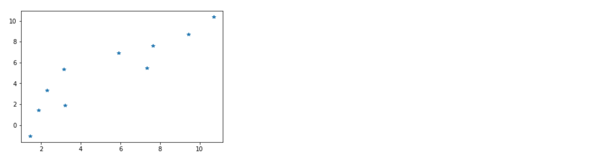
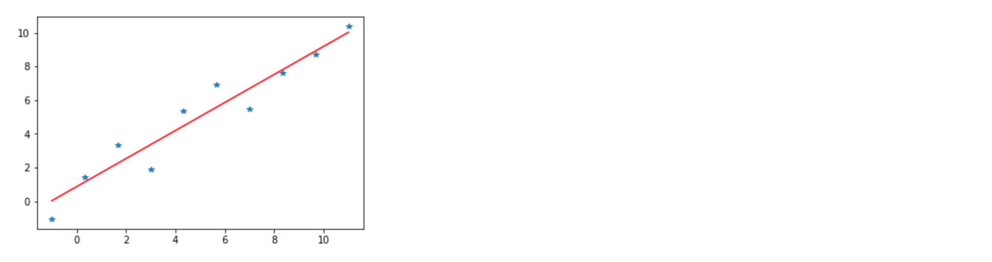
Now I want the neural network to solve $ y = mx + b$ with 10 training steps:1
2
3
4
5
6
7
8
9
10
11
12
13
14
15
16
17
18
19
20
21
22
23
24
25
26
27# create two random variables
m = tf.Variable(0.44)
b = tf.Variable(0.87)
error = 0 # create an error starting from 0
for x,y in zip(x_data, y_label): # zip makes a list of x,y
y_hat = m * x + b
error += (y - y_hat) ** 2 # cost function
optimizer = tf.train.GradientDescentOptimizer(learning_rate = 0.001)
train = optimizer.minimize(error)
init = tf.global_variables_initializer()
with tf.Session() as sess:
sess.run(init)
training_steps = 10
for i in range(training_steps):
sess.run(train)
final_slope, final_intercept = sess.run([m,b])
# Test
x_test = np.linspace(-1,11,10)
y_pred = final_slope * x_test + final_intercept
plt.plot(x_test, y_pred, 'r')
plt.plot(x_test, y_label,'*')
TensorFlow Regression
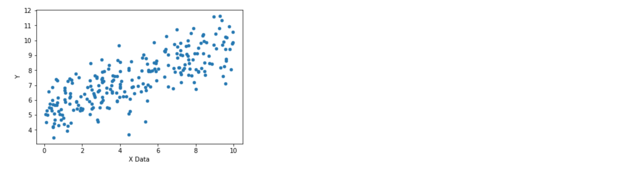
Regression example with huge dataset:1
2
3
4
5
6
7
8
9
10
11
12
13
14
15
16import numpy as np
import pandas as pd
import matplotlib.pyplot as plt
%matplotlib inline
import tensorflow as tf
x_data = np.linspace(0.0,10.0,1000000) # huge dataset
noise = np.random.randn(len(x_data)) # add noise
# y = mx + b | b = 5, m = 0.5
y_true = (0.5 * x_data) + 5 + noise
x_df = pd.DataFrame(data = x_data, columns = ['X Data'])
y_df = pd.DataFrame(data = y_true, columns = ['Y'])
my_data = pd.concat([x_df, y_df], axis = 1) # axis = 1 column concatenate
my_data.sample(n = 25) # random 25 samples
my_data.sample(n=250).plot(kind = 'scatter', x = 'X Data', y = 'Y')
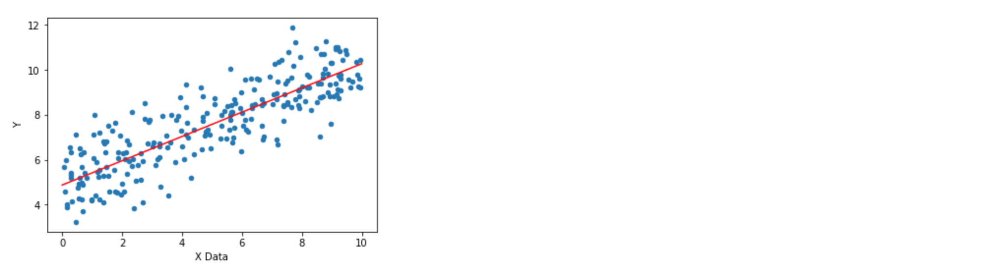
For real cases, usually the datasets are humongous and we do not use all of them at once. Instead, we use batch method to feed the data batch by batch into the network to save the time. The number of batches depends on the size of the data. Here we feed 1000 batches of data, with each batch has 8 corresponding data points (x data points with corresponding y labels). To make batches useful, we grab 8 random data points via rand_ind = np.random.randint(len(x_data), size = batch_size), then train the optimizer.1
2
3
4
5
6
7
8
9
10
11
12
13
14
15
16
17
18
19
20
21
22
23
24
25
26
27batch_size = 8
m = tf.Variable(0.81)
b = tf.Variable(0.17)
xph = tf.placeholder(tf.float32,[batch_size])
yph = tf.placeholder(tf.float32,[batch_size])
y_model = m * xph + b # the Graph I want to compute
# Loss function
error = tf.reduce_sum(tf.square(yph - y_model)) # tf.reduce_sum: Computes the sum of elements across dimensions of a tensor.
# Optimizer
optimizer = tf.train.GradientDescentOptimizer(learning_rate = 0.001) # This is gradient decent optimizer, there are many other optimizers
train = optimizer.minimize(error)
init = tf.global_variables_initializer()
with tf.Session() as sess:
sess.run(init)
batches = 1000
for i in range(batches):
rand_ind = np.random.randint(len(x_data), size = batch_size) # random index
feed = {xph: x_data[rand_ind], yph: y_true[rand_ind]}
sess.run(train, feed_dict = feed)
model_m, model_b = sess.run([m, b])
y_hat = x_data * model_m + model_b
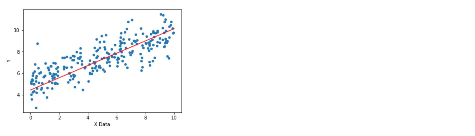
my_data.sample(250).plot(kind = 'scatter', x = 'X Data', y = 'Y')
plt.plot(x_data, y_hat, 'r')
TensorFlow Estimator API
This section is to solve the regression task with TensorFlow estimator API. Wait a minute, what is API? Technically, API stands for Application Programming Interface, but still, what is that? Basically, it is part of the server, that can be distinctively separated from its environment, that receives requests and sends responses. Here is an excellent article from Petr Gazarov explaining API.
There are many other higher levels of APIs (Keras, Layers…). The tf.estimator API has several model types to choose from:
- tf.estimator.LinearClassifier: Constructs a linear classification model
- tf.estimator.LinearRegressor: Constructs a linear regression model
- tf.estimator.DNNClassifier: Constructs a neural network classification model
- tf.estimator.DNNRegressor: Constructs a neural network regression model
- tf.estimator.DNNLinearCombinedRegressor: Constructs a neural network and linear combined regression model
Steps for using the Estimator API:
- Define a list of feature columns
- Create the Estimator Model
- Create a Data Input Function
- Call train, evaluate, and predict methods on the estimator object
1 | feat_cols = [tf.feature_column.numeric_column('x', shape = 1)] # set all feature columns |
Output:Training data matrics
{'loss': 8.7310658, 'average_loss': 1.0913832, 'global_step': 1000}
Test data matrics
{'loss': 8.6690454, 'average_loss': 1.0836307, 'global_step': 1000}
This is a good way to check if the model is overfitting (very low loss on training data but very high loss on test data). We want the loss of training data and test data are very close to each other.1
2
3
4
5# Get predict value
brand_new_data = np.linspace(0,10,10)
input_fn_predict = tf.estimator.inputs.numpy_input_fn({'x': brand_new_data}, shuffle = False)
estimator.predict(input_fn = input_fn_predict)
list(estimator.predict(input_fn = input_fn_predict))
Output:[{'predictions': array([ 4.43396044], dtype=float32)},
{'predictions': array([ 5.06833887], dtype=float32)},
{'predictions': array([ 5.7027173], dtype=float32)},
{'predictions': array([ 6.33709526], dtype=float32)},
{'predictions': array([ 6.97147369], dtype=float32)},
{'predictions': array([ 7.60585213], dtype=float32)},
{'predictions': array([ 8.24023056], dtype=float32)},
{'predictions': array([ 8.87460899], dtype=float32)},
{'predictions': array([ 9.50898743], dtype=float32)},
{'predictions': array([ 10.14336586], dtype=float32)}]1
2
3
4
5
6# plot the prediction
predictions = []
for pred in estimator.predict(input_fn = input_fn_predict):
predictions.append(pred['predictions'])
my_data.sample(250).plot(kind = 'scatter', x = 'X Data', y = 'Y')
plt.plot(brand_new_data, predictions, 'r')
TensorFlow Classification
Use real dataset “Pima Indians Diabetes Dataset”, including both categorical and continuous features, to use tf.estimator switching models – from linear classifier to dense neural network classifier.
Linear Classifier
1 | diabetes = pd.read_csv('pima-indians-diabetes.csv') |
1
diabetes.columns
Output: Index(['Number_pregnant', 'Glucose_concentration', 'Blood_pressure', 'Triceps',
'Insulin', 'BMI', 'Pedigree', 'Age', 'Class', 'Group'],
dtype='object')1
2
3
4
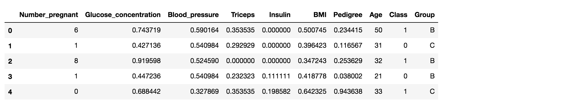
5# normalize the data except the catagorical part (Age, Class, Group)
cols_to_norm = ['Number_pregnant', 'Glucose_concentration', 'Blood_pressure', 'Triceps',
'Insulin', 'BMI', 'Pedigree']
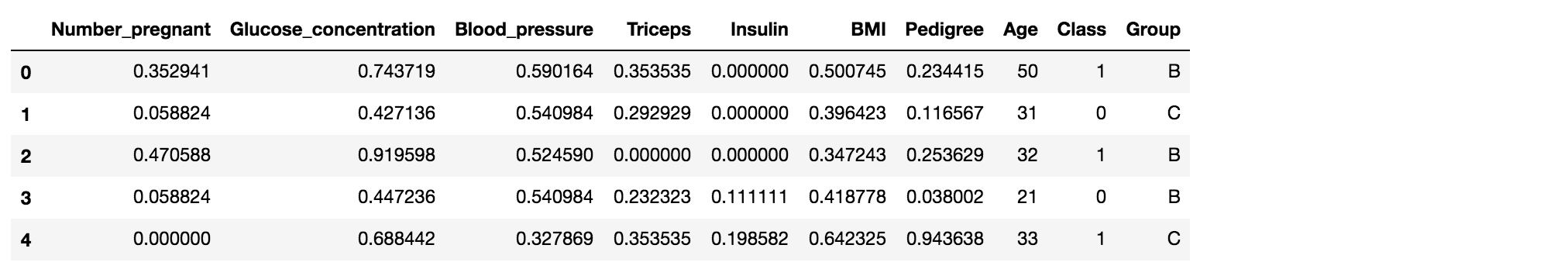
diabetes[cols_to_norm] = diabetes[cols_to_norm].apply(lambda x: (x - x.min())/(x.max() - x.min()))
diabetes.head()
1
2
3
4
5
6
7
8
9
10
11
12
13
14
15
16
17# create feature columns
# continuous value
num_preg = tf.feature_column.numeric_column('Number_pregnant')
plasma_gluc = tf.feature_column.numeric_column('Glucose_concentration')
dias_press = tf.feature_column.numeric_column('Blood_pressure')
tricep = tf.feature_column.numeric_column('Triceps')
insulin = tf.feature_column.numeric_column('Insulin')
bmi = tf.feature_column.numeric_column('BMI')
diabetes_pedigree = tf.feature_column.numeric_column('Pedigree')
age = tf.feature_column.numeric_column('Age')
# catagorical value
assigned_group = tf.feature_column.categorical_column_with_vocabulary_list('Group', ['A','B','C','D'])
# assigned_group = tf.feature_column.categorical_column_with_hash_bucket('Group', hash_bucket_size = 10)
# For many groups scenario we can use hash_bucket, as long as we set the hash_bucket_size > # of groups
import matplotlib.pyplot as plt
%matplotlib inline
diabetes['Age'].hist(bins = 20)
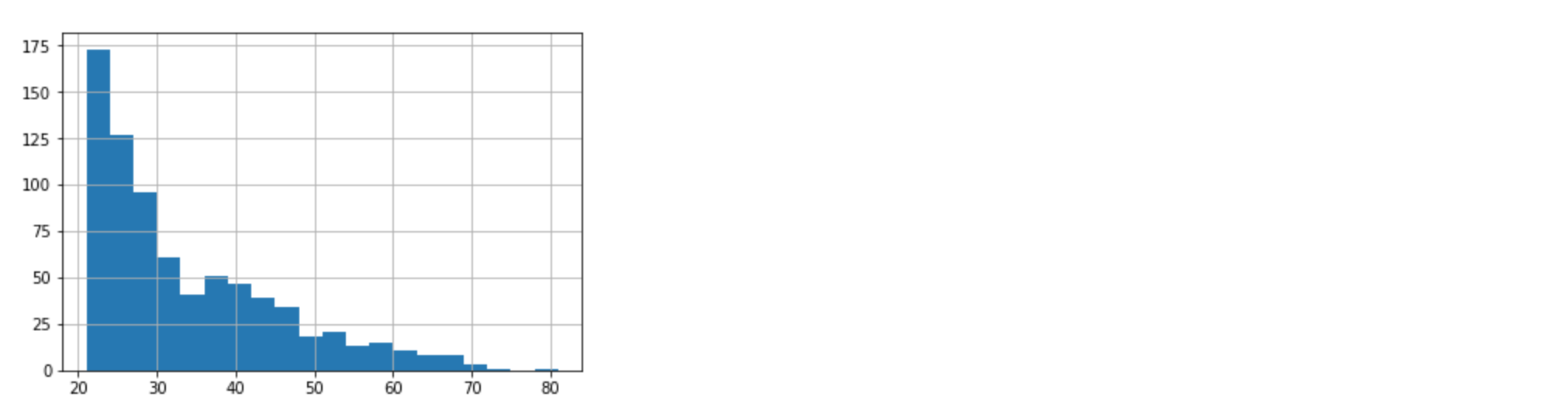
The distribution of Age from the histgram shows that most of the people are 20s. And instead of treating this variable as a continuous variable, we can bucket these values together, making boundary for each decade or so. Basically we use bucket system to transform continuous variable into categorial variable.1
2
3
4
5
6
7
8age_bucket = tf.feature_column.bucketized_column(age, boundaries = [20,30,40,50,60,70,80])
# feature columns
feat_cols = [num_preg ,plasma_gluc,dias_press ,tricep ,insulin,bmi,diabetes_pedigree ,assigned_group, age_bucket]
# train test split
x_data = diabetes.drop('Class', axis = 1) # Class column is Y
labels = diabetes['Class']
from sklearn.model_selection import train_test_split
X_train, X_test, y_train, y_test = train_test_split(x_data, labels, test_size = 0.3, random_state = 101)
Create the model!1
2
3
4
5
6
7
8## Create the model
input_func = tf.estimator.inputs.pandas_input_fn(x = X_train, y = y_train, batch_size = 10, num_epochs = 1000, shuffle = True)
model = tf.estimator.LinearClassifier(feature_columns = feat_cols, n_classes = 2)
model.train(input_fn = input_func, steps = 1000)
## Evaluate the model
eval_input_func = tf.estimator.inputs.pandas_input_fn(x = X_test, y = y_test, batch_size = 10, num_epochs = 1, shuffle = False)
results = model.evaluate(eval_input_func)
results
Output:{'accuracy': 0.73160172,
'accuracy_baseline': 0.64935064,
'auc': 0.79658431,
'auc_precision_recall': 0.6441071,
'average_loss': 0.52852213,
'global_step': 1000,
'label/mean': 0.35064936,
'loss': 5.0870256,
'prediction/mean': 0.35784912}
The accuracy is 73.16%.
Prediction!
1
2
3
4
5# No y value in prediction, put new data set in x
pred_input_func = tf.estimator.inputs.pandas_input_fn(x = X_test, batch_size = 10, num_epochs = 1, shuffle = False)
predictions = model.predict(pred_input_func)
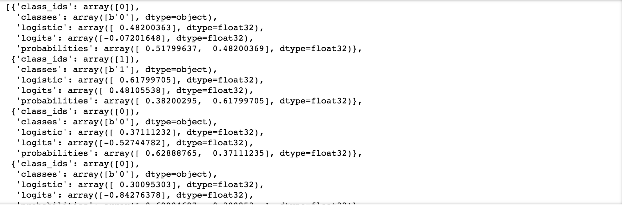
my_pred = list(predictions)
my_pred
Dense Neural Network Classifier
1 | # Create a three-layer neural network, with 10 neurons in each layer |
Output:{'accuracy': 0.75757575,
'accuracy_baseline': 0.64935064,
'auc': 0.82814813,
'auc_precision_recall': 0.67539084,
'average_loss': 0.49014509,
'global_step': 1000,
'label/mean': 0.35064936,
'loss': 4.7176466,
'prediction/mean': 0.36287409}