This chapter gives basic introduction of Vapnik-Chervonenkis Theory on Binary Classification. When it comes to binary classification task, we always want to know the functional relationship between $\mathbf{x}$ and $y$, or how to determine the “best” approach to determining from the available observaions such that given a new observation $\mathbf{x}^{new}$, we can predict its class $y^{new}$ as accurately as possible.
Universal Best
Constructing a classification rule that puts all the points in their corresponding classes could be dangerous for classifying new observations not present in the current collection of observations. So to find an classification rule that achieves the absolute very best on the present data is not enough since infinitely many more observations can be generated. Even the universally best classifier will make mistakes.
Of all the functions in $\mathcal{Y}^{\mathcal{X}}$, assume that there is a function $f^*$ that maps any $\mathbf{x}\in\mathcal{X}$ to the corresponding $y\in\mathcal{Y}$ with the minimum number of mistakes. $f^*$ is denoted as universal best
$$\begin{align*}
f^* :\quad & \mathcal{X} \rightarrow \mathcal{Y}\\
& \mathbf{x} \rightarrow f^*(\mathbf{x})
\end{align*}$$
$f$ denote any generic function mapping an element $\mathbf{x}$ of $\mathcal{X}$ to its corresponding image $f(\mathbf{x})$ in $\mathcal{Y}$. Each time $\mathbf{x}$ is drawn from $\mathbb{P}(\mathbf{x})$, the disagreement between the image $f(\mathbf{x})$ and the true image y is called the loss, denoted by $l(y, f(\mathbf{x}))$. The expected value of this loss function with respect to the distribution $\mathbb{P}(\mathbf{x})$ is called the risk functional of $f$, denoted as $R(f)$.
$$ R(f) = \mathbb{E}[l(Y, f(\mathbf{X}))] = \int l(y, f(\mathbf{x})) d \mathbb{P}(\mathbf{x}) $$
The best function $f^*$ over the space $\mathcal{Y}^{\mathcal{X}}$ of all measurable functions from $\mathcal{X}$ to $\mathcal{Y}$ is therefore
$$\begin{align*}
f^* &=\texttt{arg} \underset{f}{inf} R(f) \\
R(f^*) &= R^* = \underset{f}{inf} R(f)
\end{align*}$$
Note: Finding $f^*$ without the knowledge of $\mathbb{P}(\mathbf{x})$ means having to search the infinite dimensional function space $\mathcal{Y}^{\mathcal{X}}$ of all mappings from $\mathcal{X}$ to $\mathcal{Y}$, which is an ill-posed and computationally nasty problem (No way to get the universal best).
Thus, we seek a more reasonable way to solve the problem via choosing from a function space $F\subset \mathcal{Y}^{\mathcal{X}} $ , a function $f^+ \in F$ that best estimates the dependencies between $\mathbf{x}$ and $y$. The goal of statistical function estimation is to devise a technique (strategy) that chooses from the function class $\mathcal{F}$, the one function whose true risk is as close as possible to the lowest risk in class $\mathcal{F}$. So it is crucial to define what is meant to be best estimates. Hence we need to know what is loss function and risk functional.
Loss Functioin and Risk Functional
For classification task, the so-called 0-1 loss function defined below is used.
$$ l(y, f(\mathbf{x})) = \mathbb{1}_{Y\neq f(X)} = \begin{cases} 0, &\text{if } y = f(\mathbf{x}) \\ 1, &\text{if } y \neq f(\mathbf{x}) \end{cases} $$
And the corresponding risk functional, also named cost function showed below confirms the intuition because it is estimated in practice by simply computng the proportion of misclassfied entities.
$$ R(f)= \int l(y, f(\mathbf{x})) d \mathbb{P}(\mathbf{x}) = \mathbb{E}[\mathbb{1}_{Y\neq f(X)}] = \underset{(X,Y)\sim \mathbb{P}}{Pr}[Y\neq f(X)]$$
The minimizer of the 0-1 risk functional over all possible classifiers is the so-called Bayes classifier which we shall denote here by $f^*$. It minimizes the rate of misclassifications.
$$ f^* =\texttt{arg} \underset{f}{inf} R(f) = \texttt{arg} \underset{f}{inf} [\underset{(X,Y)\sim \mathbb{P}}{Pr}[Y\neq f(X)] ]$$
Specifically, the Bayes’ classifier $f^*$ is given by the posterior probability of class membership, namely
$$ f^* =\texttt{arg} \underset{y\in \mathcal{Y}}{max} [Pr[Y=y | \mathbf{x}] ]$$
Because it is impossible to find the universal best $f^*$, We need to select a reasonable function space $F\subset \mathcal{Y}^{\mathcal{X}} $, and then choose the best estimator $f^+$ from $\mathcal{F}$. For the binary pattern recognition problem, one may consider finding the best linear separating hyperplane.
For empirical risk minimization,
$$\begin{align*}
\hat{R}(f) &= \frac{1}{n}\sum_{i=1}^n \mathbb{1}_{Y\neq f(X)}\\
\hat{f} &= \underset{f\in \mathcal{F}}{\texttt{argmin}} [ \frac{1}{n}\sum_{i=1}^n \mathbb{1}_{Y\neq f(X)} ]
\end{align*}$$
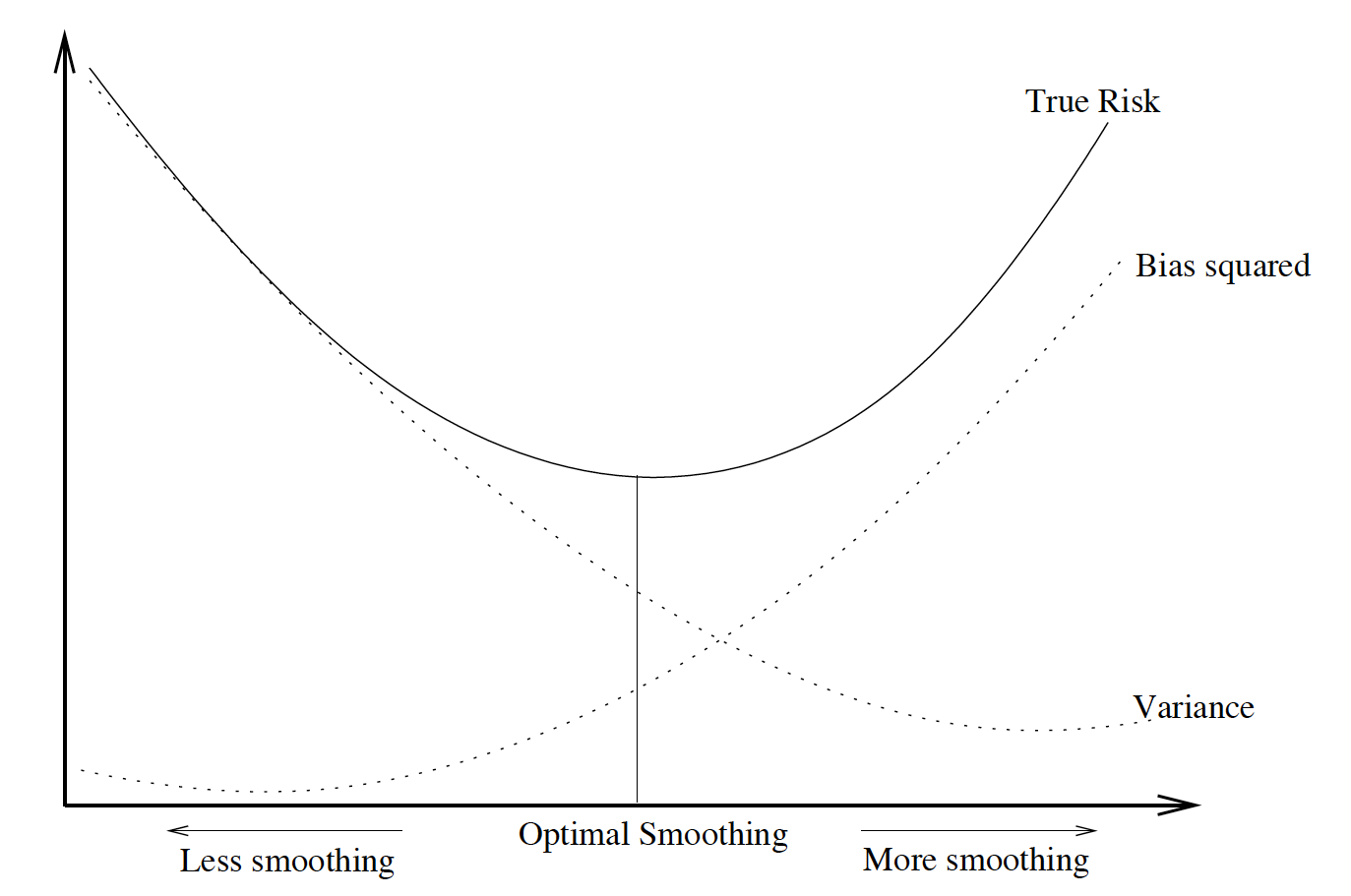
Bias-Variance Trade-Off
In statistical estimation, the blow important issues needs to be taken into account:
- Bias of the estimator
- Variance of the estimator
- Consistency of the estimator
In point estimation, given $\theta$ as the true value of the parameter, $\hat{\theta}$ is a point estimator of $\theta$, then the total error can be decomposed as: $$\begin{align*} \hat{\theta}-\theta = \underbrace{ \hat{\theta}- \mathbb{E}[ \hat{\theta}]}_\text{Estimation error} + \underbrace{\mathbb{E}[ \hat{\theta}]-\theta}_\text{Bias} \end{align*}$$ Under the squared error loss, one seeks $\hat{\theta}$ that minimizes the mean squared error, rather than trying to find the minimum variance unbiased estimator (MVUE).$$\begin{align*} \hat{\theta}=\underset{\theta\in \Theta}{\texttt{argmin}}\mathbb{E}[ (\hat{\theta}-\theta)^2] = \underset{\theta\in \Theta}{\texttt{argmin}}MSE(\hat{\theta}) \end{align*}$$ Actually, the traditional bias-variance decomposition of the MSE reveals the bias-variance trade-off: $$\begin{align*} MSE(\hat{\theta}) &= \mathbb{E}[ (\hat{\theta}-\theta)^2] \\ &= \mathbb{E}[ (\hat{\theta}- \mathbb{E}[ \hat{\theta}])^2] + \mathbb{E}[(\mathbb{E}[ \hat{\theta}]-\theta)^2 ] \\ &= \text{Variance} + \text{Bias}^2 \end{align*}$$ Again becasue of the previous statement that we cannot get the true value of $\theta$, MVUE will not help, which means the estimation we get contains bias. If the bias is too small, variance would be very large. Vice versa. The best compromise is then to trade-off bias and variance. In functional terms we call it trade-off between approximation error and estimation error.
Statistical Consistency
$\hat{\theta}_n$ is a consistent estimator of $\theta$ if $\forall \epsilon >0$
$$ \underset{n\rightarrow \infty}{lim}Pr[|\hat{\theta}_n-\theta|>\epsilon] = 0 $$
It turns out that for unbiased estimators $\hat{\theta}_n$, consistency is straightforward as direct consequence of a basic probabilistic inequality like Chebyshev’s inequality. However, for biased estimators, one has to be more careful.
The ERM (Consistency of the Empirical Risk Minimization) principle is consistent if it provides a sequence of functions for which both the expected risk and the empirical risk converge to the minimal possible value of the risk in the function class under consideration.
$$\begin{align*}
R(\hat{f}_n) & \xrightarrow[n \rightarrow \infty]{P} \underset{f\in \mathcal{F}}{inf}R(f) = R(f^+) \\
\underset{n\rightarrow \infty}{lim} Pr&[\underset{f\in\mathcal{F}}{sup}|R(f)-\hat{R}_n(f)|>\epsilon] = 0
\end{align*}$$
As $\hat{R}_n(f) $ reveals the disagreement between classifier $f$ and the truth about the label $y$ of $\mathbf{x}$ based on information contained in the sample $\mathcal{D}$. So for a given (fixed) function (classifier) $f$,
$$ \mathcal{E}[\hat{R}_n(f)] = R(f) $$
Key Question:
Since one cannot calculate the true error, how can one devise a learning strategy for choosing classifiers based on it?
Tentative Answer:
At least devise strategies that yield functions for which the upper bound on the theoretical risk is as tight as possible:
With probability $1 − \delta$ over an i.i.d. draw of some sample according to the distribution $\mathcal{P}$, the expected future error rate of some classifier is bounded by a function $g$ ($\delta$, error rate on sample) of $\delta$ and the error rate on sample. $\Downarrow\Downarrow\Downarrow$
$$\begin{align*}
\text{Pr}\Big\{ \texttt{TestError} \leq \texttt{TrainError} + \phi(n,\delta, \kappa (\mathcal{F})) \Big\} \leq 1-\delta
\end{align*}$$
Thorem: (Vapnik and Chervonenkis, 1971)
Let $\mathcal{F}$ be a class of functions implementing so learning machines, and let $\xi = VCdim(\mathcal{F})$ be the VC dimension of F. Let the theoretical and the empirical risks be defined as earlier and consider any data distribution in the population of interest. Then $\forall f\in \mathcal{F}$, the prediction error (theoretical risk) is bounded by
$$ R(f) \leq \hat{R}_n(f) + \sqrt{ \frac{\zeta(\text{log}\frac{2n}{\zeta}+1)-\text{log}\frac{\eta}{4} }{n}} $$
with probability of at least $1-\eta$. or
$$\text{Pr} \Big( \texttt{TestError} \leq \texttt{TrainError} + \sqrt{ \frac{\zeta(\text{log}\frac{2n}{\zeta}+1)-\text{log}\frac{\eta}{4} }{n}} \Big) \leq 1-\eta $$
VC Bound
- From the expression of the VC Bound, to improve the predictive performance (reduce prediction error) of a class of machines is to achieve a
trade-off (compromise) between small VC dimension and minimization of the empirical risk. - One of the greatest appeals of the VC bound is that, though applicable to function classes of infinite dimension, it preserves the same intuitive form as the bound derived for finite dimensional $\mathcal{F}$
- VC bound is acting in a way similar to the number of parameters, since it serves as a measure of the complexity of $\mathcal{F}$.
- One should seek to construct a classifier that achieves the best trade-off between complexity of function class (measured by VC dimension) and fit to the training data (measured by empirical risk).